^{MicroStability code KINEZERO}

User's guide  

NEW 03/08/05: 

collisions included, 

mode width model improved, 

finite Larmor radius and banana width effects corrected !

Kinezero is a linear local gyrokinetic code used for microturbulence analysis. It is an eigenvalue code, therefore it can find cohabitating unstable modes, but this unables it to be extended to a non-linear version. It uses the ballooning representation, therefore it stops being valid for very low magnetic shear. Also it does not include shaping effect, it uses a s-a geometry, valid for circular cross-section. The code takes into account for ions and electrons, passing and trapped, this means that Ion Temperature Gradient modes, Trapped Electron Modes and Electon Temperature Gradient modes are computed. The impact of collisions on the trapped electrons are included. The eigenfunction is an electrostatic potential (no magnetic perturbation included).  A gaussian function is used as a guess for the eigenfunction, this allows the code to be very fast. Indeed, it runs in about one hour on one CPU to calculate 150 growth rates, which about 380 times faster than GS2 ran in the same limit as kinezero! This rapidity allows to test extensively the impact of a large variety of parameters on the microturbulence.  

For more detailed information on the code see: C. Bourdelle, X. Garbet, G. T. Hoang, J. Ongena, R. V. Budny, Nuclear Fusion 42, 892 (2002)

Illustrations of the impact of a large variety of parameters see: slides of the training given at JET in November 2004. 

For details on the implementation of collisions see G. Regnoli, M. Romanelli, C. Bourdelle et al, EPS 2005

     Latest updates!! 25/07/05

1.      new publications

    ·       impact of density peaking at different collisionalities based on pellet injected discharges in FTU, Michele Romanelli et al , Physics of Plasmas 2004

    ·       impact of the a parameter and its role in ITB sustainement based on ITPA profiles data analysis, Clarisse Bourdelle et al, Nuclear Fusion 2005

  ·       stability analysis of JET ITBs, Yuri Baranov et al, Plasma Physics and Controled Fusion 2005

  ·       stability analysis of JET electron ITBs, G.M.D. Hogeweij et al, EPS 2005

  2.      few upgrades in the interfacing tools

     ·       Kinezero is now interfaced in JAMS at JET, you can find here the slides presented during the training session at JET in November 2004

 3.      Large upgrades in the code itself

     ·       The collisions have been added on trapped electrons thanks to Giorgio Regnoli, see his 2005 EPS paper for more details

   ·        The model used for the mode width (w) of the trial eigenfunction has been sensibly improved as can be seen on the figure below showing d/w versus s, for more details read the note.

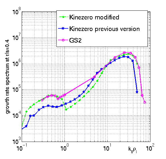
    ·        As can be seen on the comparison between Kinezero and GS2 shown in the mode width discussion, Kinezero gives lower growth rates than GS2. This difference is due to the way the bounce average of the trapped particles is treated in both codes. Kinezero simplified way of accounting for both the finite Larmor radius effects and for bounce average has now been modified in order to match better the more exact GS2 approach. Previous qualitative behaviours of the growth rates are not affected, but their absolute values are now higher and the shape of the spectra is slightly modified. More details in the note here.

    click here to view former updates, 05/03/04

Coming updates : 

None forseen at the moment, but suggestions and good will are welcome!

*** *** *** ***

To make an input file you have multiple choices, or you make it from your own data, or you read the ITPA profile database, or you make it using the Jams interface at JET :

1.      To prepare an input file with your own experimental data but this way of working is quite artisanal and not appropriate to do runs based on experimental data, it is always better to work from JETTO or so output:

·        create a kinezero directory

·        download prepkize.m or from the JAC at JET copy ~cbourde/kinezero/kizecollflr/prepkize.m

·        create a matlab file called datajet_11111_030.mat, where 11111 stands for the shot number and 030 stands for a time label such that 3s is 030, 42.34 s gives 423 and 42.36 gives 424. The file has to include :

-        B : the magnetic field in T

-        a : the minor radius in m

-        R : the major radius in m

-        x : the normalized flux surface label (ideally the normalized sqrt of the toroidal flux, or r/a)

-        te : the electron temperature in keV at each x

-        ti : the ion temperature in keV at each x

-        ne : the electron density in units of 10^19 m^-3 (ie for 4.10^19 m^-3 should be ne = 4)

-        q : the security factor at each x

-        zeff : the effective charge at each x a little smoothing of the profile is advised, otherwise you will have grad(X)/X that will jump around a bit too much, of course the big features have to be kept, so it is a delicate exercise.

·        then go in matlab and run prepkize.m, it will read the datajet file you just made, and calculate the gradients, the Larmor radii and so on. It is plotting the profiles and the associated grad(X)/X so that you can check if the smoothing was correct. For example, in an ITB, check that grad(X)/X peaks at the barrier location, or on the contrary if grad(X)/X looks very noisy, then the smoothing might have been too light leading to misleading variations of the gradients.  You will also have a plot of the electron collision frequencies compared to the electron vertical drift, nw_ge, for the minimum n and for n at k_qr_i = 2, which corresponds more or less to to upper limit of the TEM range.

·        the file containing all the needed information to run Kinezero is saved in the current directory, it is called basekinezero_11111_030.mat, where 11111 is the shot number and 030 is the time label such that 3s is 030, 42.34 s gives 423 and 42.36 gives 424.

2.    From the ITPA database

    You just need to know the tree name ('jet', 'itb_tftr', etc), the shot number you are interested in and at what time. This program reads data from the ITPA profile database.

·         create a kinezero directory

·        download mdskize.m or copy from the JAC at JET ~cbourde/kinezero/kizecollflr/mdskize.m

·        then go into matlab and run mdskize.m. It will pick up from the profile database the following data: B_tor, a, R, and the q, T_e, T_i, n_e and Z_eff profiles. It plots the profiles so that you can make sure that it is what you want to analyze. Then it calculates the gradients, Larmor radii and so on it will need in Kinezero. It plots the profiles and the associated grad(X)/X so that you can check if the smoothing was appropriate. For example, in an ITB, check that grad(X)/X peaks at the barrier location, or on the contrary if grad(X)/X looks very noisy, then the smoothing might have been too light leading to misleading variations of the gradients.  You will also have a plot of the electron collision frequencies compared to the electron vertical drift, nw_ge, for the minimum n and for n at k_qr_i = 2, which corresponds more or less to to upper limit of the TEM range.

·        the file containing all the needed information to run Kinezero is saved in the current directory, it is called basekinezero_11111_030.mat, where 11111 is the shot number and 030 is the time label such that 3s is 030, 42.34 s gives 423 and 42.36 gives 424. 

3.    Input from the JETTO output from the JAC machines at JET:

    You just need to know which shot number you are interested in and at what time. This program reads JETTO output, so you need to give the JETTO run user ID and sequence number of the shot you want to analyze.

·        create a kinezero directory

·        download jettokize.m or from the JAC at JET copy ~cbourde/kinezero/kizecollflr/jettokize.m

·         then go into matlab and run jettokize.m. It will pick up the JETTO Btor, a, R, and the q, Te, Ti, ne and Zeff profiles. It plots the profiles so that you can make sure that it is what you want to analyze. Then it calculates the gradients, Larmor radii and so on it will need in KINEZERO. It plots the profiles and the associated grad(X)/X so that you can check if the smoothing was appropriate. For example, in an ITB, check that grad(X)/X peaks at the barrier location, or on the contrary if grad(X)/X looks very noisy, then the smoothing might have been too light leading to misleading variations of the gradients. You will also have a plot of the electron collision frequencies compared to the electron vertical drift, nw_ge, for the minimum n and for n at k_qr_i = 2, which corresponds more or less to to upper limit of the TEM range.

·        the file containing all the needed information to run Kinezero is saved in the current directory, it is called basekinezero_11111_030.mat, where 11111 is the shot number and 030 is the time label such that 3s is 030, 42.34 s gives 423 and 42.36 gives 424. 

    To run Kinezero 

    ·        download kizecollflr.targz, then in unix: cp kizecollflr.targz kizecollflr.tar.gz and gunzip kizecollflr.targz and tar -xvf  kizecollflr.tar. In the makefile, correct  if necessary the links to the following libraries : libnag.a and libmat.so. Or copy from the JAC at JET in your kinezero directory ~cbourde/kinezero/kizecollflr/*.f90, makefile, *.a, *.m, kinezero.cmd

    ·        type "make", now the executable of Kinezero is ready

    ·        then addapt the kinezero.cmd batch file by: changing 11111 by the shot number, 030 by your time label, change also "cbourde" by your own user name, make sure the directory you are        sending the output is correct and set your e-mail address so that you will recieve an e-mail when the run has completed. If you want to send many jobs at the same time, save kinezero.cmd with a            different label, for example kize_11111_031.cmd.

    ·        then type: llsubmit kize_11111_030.cmd - to check if your job is running do : xloadl & then wait for the e-mail that will tell you when it is completed. If your local batch system is different from the JAC system at JET, adapt this ".cmd" file and the submition command following the recommandations of your system manager.

·        dowload plotkize.m or plotkize_omeb.m  

·        in matlab, type "plotkize", then it will ask you the shot number and the time. The 1st plot is the maximum growth rates, among the different unstable branches, versus x and the wave numbers. The matching real parts of the frequencies are also plotted in 3D, it allows to check the signs: negative means in the ion drift direction, therefore "ITG dominated", positive means in the electron drift direction, therefore "TEM dominated" or pure ETG at high wave number (n > 100). The 3rd and 4th plots are the maximum growth rates for k_qr_i < 2 (ITG-TEM range) and the maximum for k_qr_i > 2 (ETG range) versus x, accompanied by an evaluation of the contribution of trapped/passing ions/electrons in the power exchange of the most unstable mode at each radial position. Then it will ask you at what radius you want to plot the a spectrum of modes. Of course you can and should adapt this plotting tool to your convenience.

If you have a file named omExB_11111_060.mat created with mdskize.m, then you can use plotkize_omeb.m. It will also plot the ExB shearing rate read in the database with the ITG-TEM growth rates. Do not forget to check carefully how was calculated the ExB shearing rate: toridal velocity profile measured or not, etc. 

C. Bourdelle, X. Garbet, G. T. Hoang, J. Ongena, R. V. Budny, Nuclear Fusion 42, 892 (2002)

C Fourment, G T Hoang, et al Plasma Physics and Controlled Fusion 45, 233 (2003)

Michele Romanelli et al , Physics of Plasmas 2004

Clarisse Bourdelle et al, Nuclear Fusion 2005

That should be it,

for more information and help please contact Clarisse Bourdelle : mailto:clarisse.bourdelle@cea.fr , +33 (0)4 42 25 61 36.